Using the Tree of Shapes to filter an image

The Tree of Shapes (ToS) represents the inclusion relationship between the connected components of an image. Thus, a shape is a connected component with its holes filled.

The objective of this example is to show how to use the ToS to process a filtering on an image.

First, we import the needed packages

import pylena as pln
from skimage.data import camera
import matplotlib.pyplot as plt
import numpy as np
from numba import jit

Then, we load an image

img = camera()

plt.figure(figsize=(5, 5))
plt.imshow(img, cmap="gray")
plt.tight_layout()
plt.xticks([])
plt.yticks([])
plt.show()

Then, we compute the tree of shapes.

t = pln.morpho.tos(img, (0, 0))

This function computes the tree of shapes starting from the point (0, 0) of the image. However, it is usually prefered to add a border to the image, set to the median value of the pixel at the border of the image, ensuring the root is surrounding all the image.

t = pln.morpho.tos(img, (0, 0), padding="median")

This function returns a ComponentTree object. This ComponentTree class is composed of three attributes:

• nodemap: a mapping from an image pixel to a node of the tree

• parent: a maping from a node of the tree to its parent. As an example, if t.parent[4] = 1, then the parent of the node 4 is the node 1 of the tree. The parent of the node 0, corresponding to the root of the tree, is set to -1.

• values: An array assigning a value to a node. For the tree of shapes, it is the value of the pixels in the connected component related to the node.

The next step to filter the tree if to compute an attribute. In this example, the area of a shape is computed. This is already implemented in the ComponentTree class but in an objective of attribute computation explaination, it is reimplemented below

@jit(nopython=True)
def _area(parent: np.ndarray, nodemap: np.ndarray):
    res = np.zeros(parent.size)
    # 1. Compute the area of each connected component
    for it in np.nditer(nodemap):
        res[it] += 1
    # 2. Propagate to the parent nodes
    for n in range(parent.size - 1, 0, -1):  # From leaf to root
        res[parent[n]] += res[n]
    return res


def area(t: pln.morpho.ComponentTree):
    return _area(t.parent, t.nodemap)

The first function _area is divided in two parts:

• The first part compute the area of all the connected component

• The second part propagates the values to their parent. This second step is due to the fact the ToS encodes the inclusion relationship of the connected components. Each node is a shape, so its area is equal to the area of its connected components plus the areas of included shapes composing it.

It is important to note that to make the code running faster, the Numba library is used, using a Just-In-Time compiler. However, this add a limitation to the feature being used in these function. That is why another function, area is used to encapsulate _area, to make its usage easier, but it is just sugar and the _area function would be sufficient for personnal usage.

The next step is to compute the area attribute for each node of the tree

accmap = area(t)

Now the area is computed, we just need to filter the tree. To this aim, the filter method is used. The inplace argument indicates if the values table of the ComponentTree object is modified (inplace = True) or of a new array is returned. In this case, the array is copied, filtered and returned.

In our example below, only the node having an area greater than 100 are kept.

filtered_values = t.filter(accmap > 100, inplace=False)

Finally, the image is reconstructed using the reconstruct method. If no values table is provided, it uses the one inside the ComponentTree object. However, in our case, as the tree is not modified inplace, we need to provide a table or the original image will be reconstructed.

rec = t.reconstruct(filtered_values)

plt.figure(figsize=(5, 5))
plt.imshow(rec, cmap="gray")
plt.xticks([])
plt.yticks([])
plt.tight_layout()
plt.show()

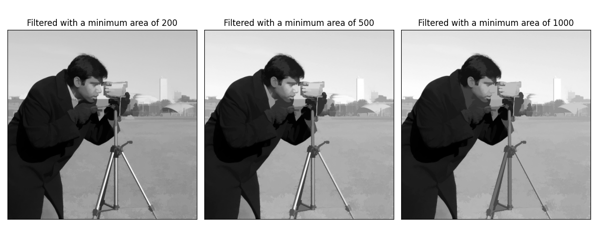
Finally, we provide some illustration using different area thresholds

i = 1
plt.figure(figsize=(12, 5))
for th in [200, 500, 1000]:
    new_values = t.filter(accmap > th, inplace=True)
    new_rec = t.reconstruct(new_values)
    plt.subplot(1, 3, i)
    plt.title(f"Filtered with a minimum area of {th}")
    plt.imshow(new_rec, cmap="gray")
    plt.xticks([])
    plt.yticks([])
    i += 1
plt.tight_layout()
plt.show()